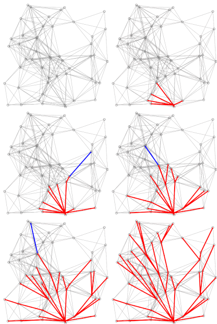
User:Jarhill/Dijkstra's algorithm
Pseudocode[edit]
In the following algorithm, the code u ← vertex in Q with min dist[u], searches for the vertex u in the vertex set Q that has the least dist[u] value. length(u, v) returns the length of the edge joining (i.e. the distance between) the two neighbor-nodes u and v. The variable alt on line 18 is the length of the path from the root node to the neighbor node v if it were to go through u. If this path is shorter than the current shortest path recorded for v, that current path is replaced with this alt path. The prev array is populated with a pointer to the "next-hop" node on the source graph to get the shortest route to the source.

 1  function Dijkstra(Graph, source):
 2
 3      create vertex set Q
 4
 5      for each vertex v in Graph:
 6          dist[v] ← INFINITY
 7          prev[v] ← UNDEFINED
 8          add v to Q
10      dist[source] ← 0
11
12      while Q is not empty:
13          u ← vertex in Q with min dist[u]
14
15          remove u from Q
16
17          for each neighbor v of u:           // only v that are still in Q
18              alt ← dist[u] + length(u, v)
19              if alt < dist[v]:
20                  dist[v] ← alt
21                  prev[v] ← u
22
23      return dist[], prev[]
If we are only interested in a shortest path between vertices source and target, we can terminate the search after line 15 if u = target. Now we can read the shortest path from source to target by reverse iteration:
1  S ← empty sequence
2  u ← target
3  if prev[u] is defined or u = source:          // Do something only if the vertex is reachable
4      while u is defined:                       // Construct the shortest path with a stack S
5          insert u at the beginning of S        // Push the vertex onto the stack
6          u ← prev[u]                           // Traverse from target to source
Now sequence S is the list of vertices constituting one of the shortest paths from source to target, or the empty sequence if no path exists.
A more general problem would be to find all the shortest paths between source and target (there might be several different ones of the same length). Then instead of storing only a single node in each entry of prev[] we would store all nodes satisfying the relaxation condition. For example, if both r and source connect to target and both of them lie on different shortest paths through target (because the edge cost is the same in both cases), then we would add both r and source to prev[target]. When the algorithm completes, prev[] data structure will actually describe a graph that is a subset of the original graph with some edges removed. Its key property will be that if the algorithm was run with some starting node, then every path from that node to any other node in the new graph will be the shortest path between those nodes in the original graph, and all paths of that length from the original graph will be present in the new graph. Then to actually find all these shortest paths between two given nodes we would use a path finding algorithm on the new graph, such as depth-first search.
Using a priority queue[edit]
A min-priority queue is an abstract data type that provides 3 basic operations : add_with_priority(), decrease_priority() and extract_min(). As mentioned earlier, using such a data structure can lead to faster computing times than using a basic queue. Notably, Fibonacci heap (Fredman & Tarjan 1984) or Brodal queue offer optimal implementations for those 3 operations. As the algorithm is slightly different, we mention it here, in pseudo-code as well :
1  function Dijkstra(Graph, source):
2      dist[source] ← 0                           // Initialization
3
4      create vertex priority queue Q
5
6      for each vertex v in Graph:
7          if v ≠ source
8              dist[v] ← INFINITY                 // Unknown distance from source to v
9              prev[v] ← UNDEFINED                // Predecessor of v
10
11         Q.add_with_priority(v, dist[v])
12
13
14     while Q is not empty:                      // The main loop
15         u ← Q.extract_min()                    // Remove and return best vertex
16         for each neighbor v of u:              // only v that are still in Q
17             alt ← dist[u] + length(u, v)
18             if alt < dist[v]
19                 dist[v] ← alt
20                 prev[v] ← u
21                 Q.decrease_priority(v, alt)
22
23     return dist, prev
Instead of filling the priority queue with all nodes in the initialization phase, it is also possible to initialize it to contain only source; then, inside the if alt < dist[v] block, the node must be inserted if not already in the queue (instead of performing a decrease_priority operation).[1]: 198
Other data structures can be used to achieve even faster computing times in practice.[2]
- ^ Cite error: The named reference
mehlhornwas invoked but never defined (see the help page). - ^ Chen, M.; Chowdhury, R. A.; Ramachandran, V.; Roche, D. L.; Tong, L. (2007). Priority Queues and Dijkstra's Algorithm – UTCS Technical Report TR-07-54 – 12 October 2007 (PDF). Austin, Texas: The University of Texas at Austin, Department of Computer Sciences.
